Simhash and solving the hamming distance problem: explained

Simhashes are a clever means of rapidly finding near-identical documents (or other items) within a large corpus, without having to individually compare every document to every other document. Using simhashes for any sizable corpus involves two parts: generating the simhash itself, and solving the Hamming distance problem. Neither is much use without the other. Unlike minhashes, the simhash approach doesn’t really allow full similarity detection, because the range of similarity it is sensitive to is so small. It’s better described as near-duplicate detection. Google have patented simhash (though not the Hamming distance solution, as far as I know).

As well as its other limitations simhash is substantially more complex than minhash and harder to tune. Its real benefit is that it performs way faster than minhash, even on enormous corpuses, and typically requires less storage.

Generating the simhash

A simhash is a single sequence of bits (usually 64 bits) generated from a set of features in such a way that changing a small fraction of those features will cause the resulting hash to change only a small fraction of its bits; whereas changing all features will cause the resulting hash to look completely different (roughly half its bits will change).

As with any similarity detection scheme, its success depends on choosing sensible features. Let’s say you’re comparing documents: a typical feature to choose might be shingles of words, with whitespacing and case normalized. You might add in other features, such as document title, text styled as headings, and so on.

Each feature must be hashed using a cheap but good standard (non-cryptographic) hash such as FNV-1a, with the same bit-length as your intended simhash.

To combine the many feature hashes into a single simhash, you calculate a kind of bitwise average of them all. It’s very simple. Take the first bit of every feature hash and average them. You get some value between 0 and 1. Round that value to 0 if it’s less than 0.5, and otherwise to 1. That gives you the first bit of your simhash. Do the same for the second bit of every feature hash, to yield the second bit of your simhash. And so on.

You can see that changing just one feature hash out of thousands may not change many (or any) bits in the simhash, whereas changing a lot of feature hashes will have a larger effect.

Comparing two documents for (estimated) similarity is now as simple as determining the Hamming distance between the two simhashes, which can be calculated very efficiently. Unfortunately, in most situations you don’t need to compare one single document to another single document; you need to compare every document to every other one. Even with such an efficient calculation of hamming distance, to find all near-duplicates in a corpus of 10 million documents would require 10M×(10M-1)/2 = nearly 50 trillion comparisons, which is completely unworkable. This is why simhashing isn’t much use without “solving the hamming distance problem”, described below. The solution to that problem only works for quite small hamming distances: typically 2 to 7 bits difference, depending on your storage capacity, speed requirements and corpus size.

For this reason, a lot of careful tuning goes into trying to make the simhashes sensitive to those features we consider most important and less sensitive to others. This involves choosing suitable features for hashing and suitable methods of normalizing features (such as lowercasing text and simplifying whitespacing). It also involves giving higher or lower weights to certain features: we thus calculate each bit of the simhash as a (rounded) weighted average.

An example of a kind of feature you might want to exclude is advertising text in a webpage. There are some simple tricks for reducing the influence of advertising text, such as only taking shingles that include at least one stopword (since advertisements typically contain few stopwords). But you may have to do more complex feature detection.

The method of calculating a simhash is described in slightly different terms in Google’s patents. As they describe it, you keep a tally for every bit, which starts at zero. For each bit of each feature hash, if it is 1, add that feature’s weight to the corresponding tally; or if it is zero subtract its weight from the tally. From the final tallies, set your simhash bit to 1 where the corresponding tally is >0, otherwise set it to 0. This is illustrated below:

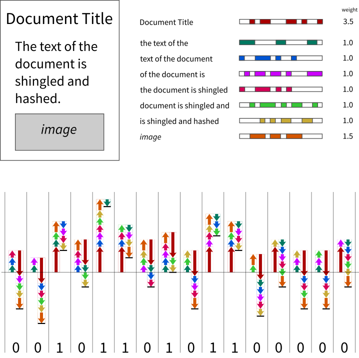
It’s a little more cumbersome to describe the algorithm this way, but it should be clear that it is exactly equivalent to a bitwise rounded weighted average.

I recommend you keep weights for particular types of feature constant. E.g., don’t weight shingles more highly near the beginning of the document and gradually less and less toward the end. Otherwise relatively small changes in position of text, such as inserting an extra paragraph early in the document, can have a substantial impact on the simhash.

There’s probably not a lot of choice in the bit-length of your simhashes. I recommend 64 bits. 128 bits would be overkill for almost any purpose, and 32 bits is insufficient for most purposes. Remember that 32 bits only stores a little over 4 billion values, which may sound like a lot, but is ripe for collisions. Let’s say your hash is 32 bits long and k is 4. For any given fingerprint there are 41,449 bit-patterns that are within k bits Hamming distance of it, and any document that happens to have one of those fingerprints as a result of a hash collision will be detected as similar. With a corpus of 100,000 documents you’d already be getting frequent collisions.

A word on images

Simhash, minhash and the like can be used for detecting similar images, if you choose sensible features to generate your feature hashes from. The features should be derived in such a way that similar images are likely to contain many identical features. This is far from straightforward. Depending on what you want to consider ‘similar’, the features may need to be robust to changes in scale, orientation, colour balance, blur/sharpness, etc.

You may want to treat images embedded in a document as features of that document, and generate simple binary hashes of them (as in the example above). If you do so, be aware that any change, visible or otherwise, will result in a different feature hash.

Solving the Hamming distance problem

Now comes the really clever bit, that relieves us of having to individually compare every simhash with every other simhash in order to find all duplicates in the corpus. This is what saves us from performing 50 trillion Hamming distance calculations to deduplicate our corpus of 10 million documents! The explanation in Google’s paper is difficult to follow, and I couldn’t find a simpler explanation, so I’m creating one here. I’ll stick to the original paper’s terminology and notation, to avoid confusion.

Let’s say we’re a Google web crawler, and we find a new document with fingerprint (simhash) F. It so happens that we’ve previously encountered another document with a very similar fingerprint G that differs by at most k=3 bits.

We can then permute these 6 blocks so that the three blocks containing differing bits all move into the low-order bits:

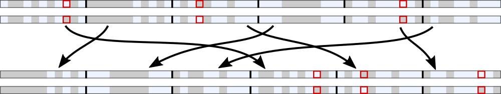
The permuted F we’ll call F′, and the permuted G we’ll call G′. Notice that in the first 3 blocks (totalling 32 bits), F′ and G′ are identical.

Now, we have kept a table of the permuted hashes of all the documents we’ve previously encountered. All the hashes in that table have had exactly the same permutation applied, and the table is sorted. That means that all the permuted hashes that share their first 32 bits with our permuted fingerprint F′ are in a single contiguous section of the table, and we can find them rapidly using binary search, or even more efficiently, interpolation search.

Once we’ve found permuted hashes that share the first 32 bits, we still need to compare the low order bits to determine total Hamming distance. Then we’ve found our similar documents.

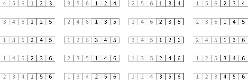
“Wait!”, I hear you say. The permutation we’ve chosen may work for this example, but what about all the other fingerprints whose 1, 2 or 3 differing bits fall in different blocks? Well, that’s why we actually store 20 such tables, each with a different permutation, so that in each table a different combination of 3 blocks is pushed into the low bits. COMB(6,3) = 20. When we look for similar fingerprints to F, we’ll have to generate 20 different permutations of it and search in each of the 20 tables.

But let’s return to F′ and G′ and this particular permuted table. Interpolation search has yielded a set of candidates that we have to calculate Hamming distance on. That’s a fairly cheap operation, but still could be time-consuming if there are a lot of candidates. So how many candidates should we expect, on average?

Well, Google indexes around 8 billion documents, which is roughly 2³⁴. So our table contains around 2³⁴ fingerprints. On average there will be just one document that shares the highest 34 bits with F′, or 4 that share the highest 32 bits (since 2^34-32 = 4). So on average, we’ll only have to calculate hamming distance for 4 candidates (within this table). Nice!

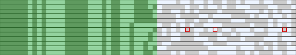
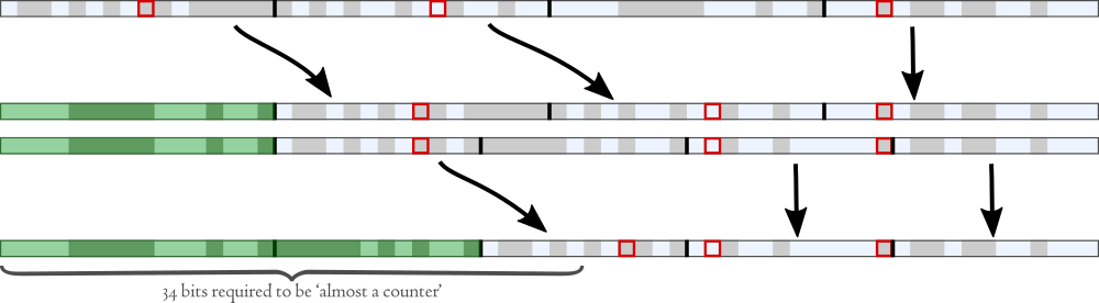
There’s another way to explain this: Imagine we have 2³⁴ truly random fingerprints, in sorted order. If we take just the first 34 bits of these fingerprints (shaded green below), they will amount to ‘almost a counter’, since most of the possible numbers will be represented and only a minority of possible numbers will be repeated. If we take just the least significant 30 bits, though, they will look “almost random”.

But we’re only matching the first 32 bits, so we find on average 4 candidates per query.

Because 64 isn’t evenly divisible by 6, our blocks are 11, 11, 11, 11, 10 and 10 bits wide. That means our different tables will need to be searched with different numbers of high-end bits: 31, 32 or 33 depending on the permutation, yielding 8, 4 or 2 candidates on average.

By performing this same cheap search on each of the 20 tables we can be certain we have found every fingerprint that differs by at most k=3 bits.

Storing the tables

For fast response, tables should be held in main memory. Each of the permuted tables should store only permuted hashes, and a separate table should contain mappings from the unpermuted hashes back to document IDs.

The most compact storage for the hash tables is as a sorted list (and Google’s paper describes how to further compress the table). If you want to insert new entries as you go then you’ll need trees (quite a bit more storage required), or else you could keep most entries in sorted lists and new entries in trees and check both, and periodically merge the trees back into the sorted lists.

If you don’t have to detect similarities as soon as new documents arrive, there are nice efficiencies to be gained. Not only can you store the tables as more compact sorted lists, you can also find all similarities in a single pass through all tables, by just finding every group of permuted hashes that shares the first d bits, and checking their Hamming distances.

In Google’s paper they recommend a means of compacting a sorted list still further, exploiting the fact that many of the high-end bits don’t change much from one entry to the next. I’ve never bothered with this, but if you’re really struggling with storage, bear it in mind.

Other configurations

Aside from the 6-block configuration discussed above, there are other configurations that give different memory/processing trade-offs with k=3. For instance, 4 blocks (of 16 bits each) requires only 4 permuted tables (since COMB(4,3) = 4).

Given there are only 16 bits we are doing the table search on, we can expect on average 2^34-16 = 262,144 results per query for each table, or about a million hamming checks per query overall.

In the example above, we match on 16 bits, leaving 48 non-match bits. We could further subdivide each table, by splitting the 48 non-match bits into 4 blocks of 12 bits each and permuting them in turn, for a total of 16 tables:

Now we can match on the first 28 bits, using 16 tables and getting on average 2^34-28 = 64 results per query.

There are several such table variants described in Google’s paper, each offering a different trade-off between number of tables required, and average number of candidate matches per query.

Many applications won’t need to index 2³⁴ documents, and could increase k a little. For instance, let’s say you only expect to index around 2²³ (~8 million) documents. You could readily increase the possible Hamming distance up to k = 6, by dividing the hash into 8 blocks (28 tables). On average you’d be getting 128 candidates per query for each table, meaning you’d have to perform about 3,500 hamming distance checks in total per query.

You will need to find a table arrangement that works best for you. Decide on the bit-length of your simhashes; test the simhashes you produce from your documents to determine how many bits of Hamming distance you need to allow (k); and determine how large your corpus is expected to grow and thus how many bits would be “almost a counter”. Then you can figure out a suitable permutation scheme that balances storage size against processing time.

If you find that you need to detect more bits difference than this approach can accommodate, you are probably looking for full similarity detection rather than near-duplicate detection, and should investigate algorithms such as minhash.